
One command:
python generate.py --task t2v-A14B --size 1280*720 \
  --ckpt_dir ./Wan2.2-T2V-A14B --prompt "Two anthropomorphic cats boxing"
A few minutes later, you get an 81-frame, 720p, 16fps video. This article explains every step that happens in between. All code comes from the original Wan2.2 repository, and every number can be calculated from the configuration files; I include the formulas as well. After reading it, you should be able to answer these questions:
- Why must the frame count be 4n+1, and why won’t 80 frames work?
- How is the 14B parameter count derived from the configuration? How is the 80GB VRAM threshold calculated?
- Mathematically, how does flow matching differ from DDPM, and why can the former produce videos in just 40 steps?
- What knob does
--sample_shift 12turn, and what invisible linkage does it have with MoE expert switching? - For image-to-video, which exact lines are changed on top of the text-to-video backbone?
The full article follows the order of “principles → data → network → sampling → engineering.” Each chapter only uses concepts introduced in the previous chapters, so I recommend reading it sequentially. I assume you roughly know what tensors and attention are; if you are starting completely from scratch, spend ten minutes looking up those two terms first. Those ten minutes are worth it.
Three Models, One Stage
Video generation is not done by one model, but three:
| Model | Role | In Wan2.2 t2v-A14B |
|---|---|---|
| Text encoder | Turns the prompt into a sequence of vectors | The encoder of umT5-XXL, about 5.7B parameters |
| Diffusion backbone | Step by step, “carves” a compressed representation of the video out of noise | WanModel, DiT architecture, 40 layers, 14B parameters × 2 experts |
| VAE | Translates back and forth between pixels and compressed representations | Wan2_1_VAE, spatiotemporal compression ratio 4×8×8 |
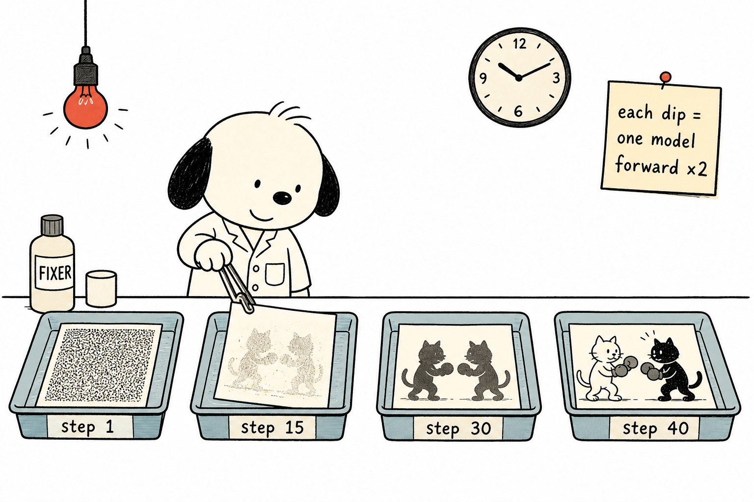
Let’s first cushion the word “diffusion” with three sentences, then expand on it in Chapter 1: what the model learns is the direction for “repairing a block of noise toward clean data”; during inference, it starts from pure random noise, asks the model for a direction 40 times, moves 40 times, and the noise gradually develops into a video; your prompt participates in every direction judgment. Remember this skeleton, and every component later can hang on it.
The division of labor is clear: T5 only runs once at the beginning; the VAE encoder is not used at all in t2v, because there is no input image; the decoder only runs once at the end. What really burns compute is the diffusion backbone in the middle: it has to run for 40 steps, with two forward passes per step. Why two? Chapter 5 will cover that.
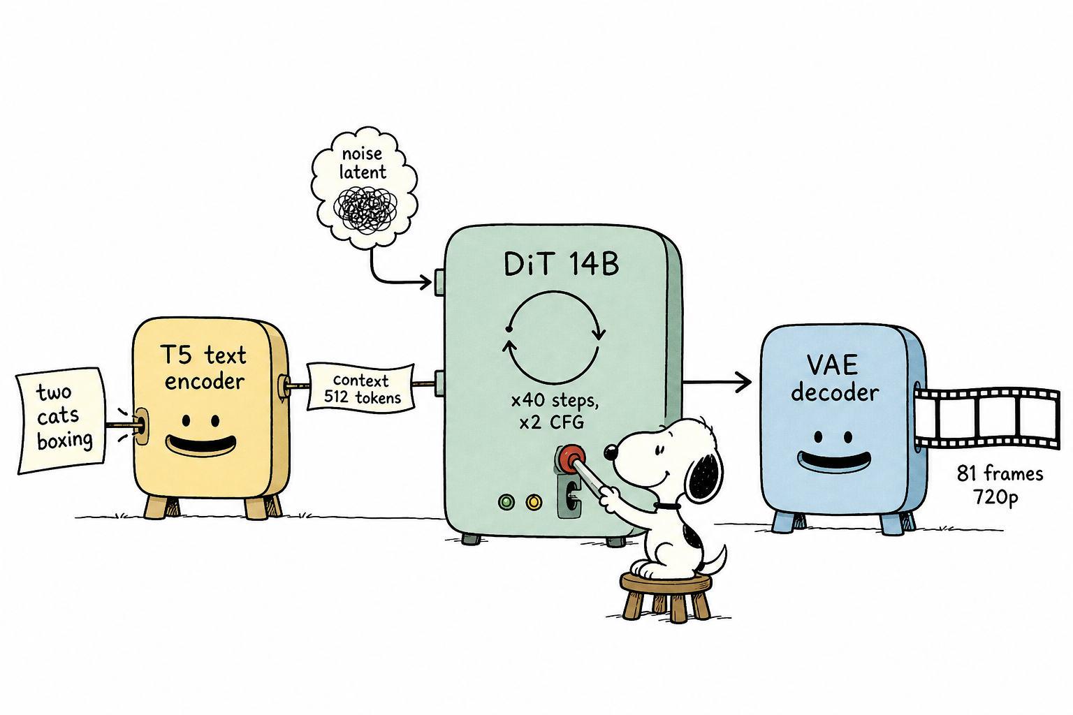
How the three models are connected is scripted in generate() in wan/text2video.py: encode text → sample noise → loop denoising → decode into pixels. It is worth memorizing the skeleton of this script first; every later chapter expands on one of its lines.
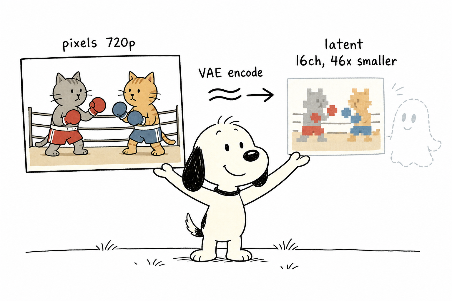
First, let’s resolve a prerequisite question: why doesn’t diffusion operate directly on pixels? Do the math. An 81-frame 720p RGB video has
81 × 720 × 1280 × 3 ≈ 224 million values
After VAE compression, the latent only has
16 × 21 × 90 × 160 ≈ 4.84 million values
That is 46× fewer. The diffusion backbone has to repeatedly compute over this block of data for 80 forward passes. With the data 46× smaller, the cost of both attention and convolution collapses along with it. Generating in compressed space and decoding back to pixels only in the final step is called latent diffusion. It became standard starting with Stable Diffusion, and video generation extends it from 2D to 3D.
Chapter 1: Denoising Takes a Straight Line
Before looking at any code, let’s settle the most fundamental question: why can “fixing noise step by step” generate a brand-new video out of thin air?
Why “Add Noise, Then Denoise” Can Generate
The problem a generative model needs to solve is: sample a new example from the “distribution of natural videos.” This distribution has no analytical form, so there is no direct way to sample from it. Diffusion methods take this approach: build a road whose two ends are natural data and standard Gaussian noise—the latter is easy to sample—then train a network to walk back along this road from the noise end to the data end. The noising process is road construction: it connects a complex distribution to a simple one. The denoising network learns, at every position on this road, “which direction should I move to get closer to data.” During training, the network sees massive numbers of “position → direction” examples. During inference, it starts from random noise and follows the learned direction field. The endpoint is a new sample that looks like the training data, but is not identical to any training example. The prompt participates in the direction decision at every step—the concrete mechanism appears in Chapters 3 and 4—constraining the endpoint to the region that “matches this description.”
From DDPM to Flow Matching
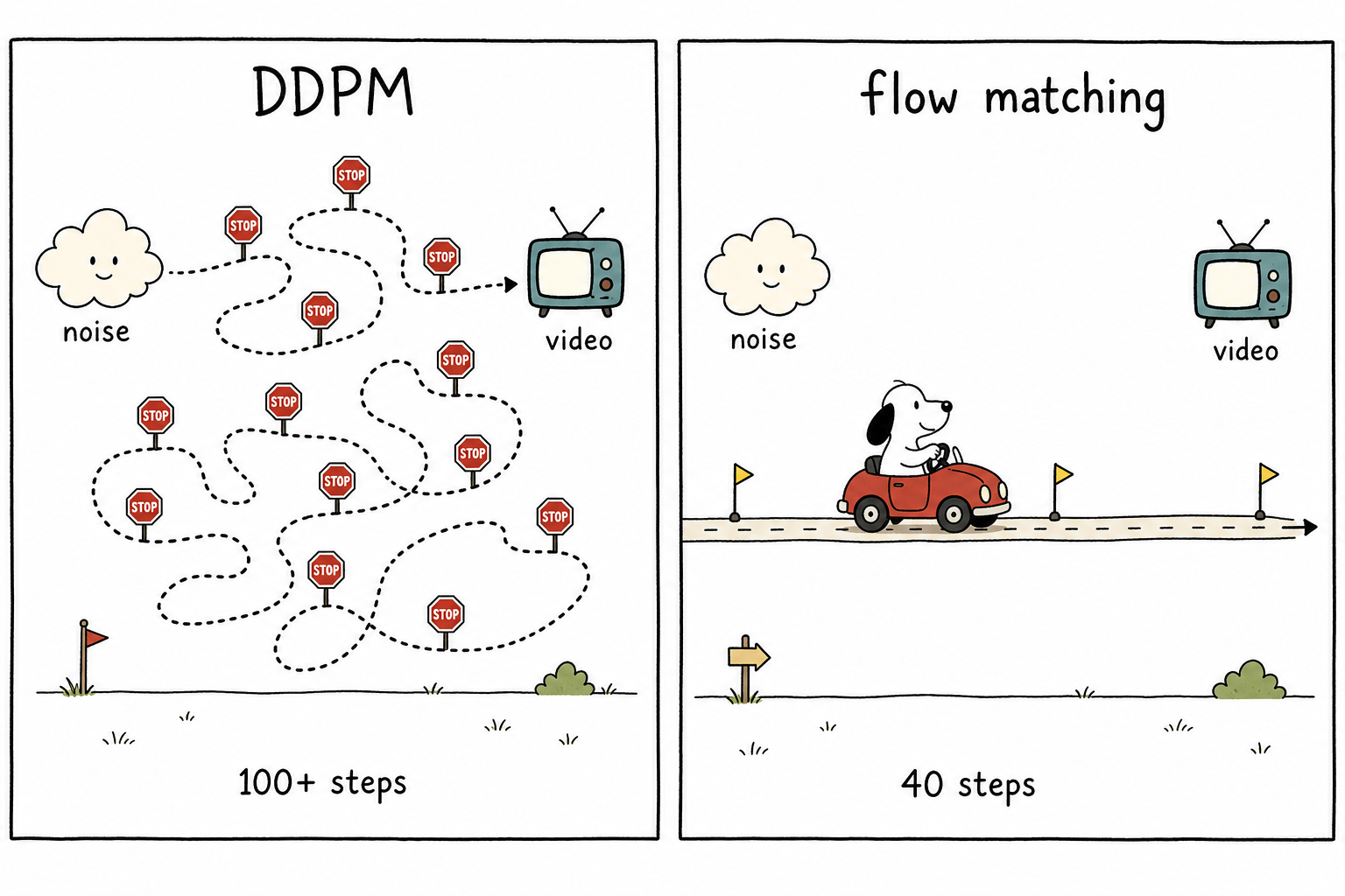
Classic DDPM defines this road like this: the forward process gradually adds Gaussian noise according to a carefully designed variance schedule; the reverse process trains a network to predict the noise added at each step; and sampling peels it away step by step using Bayes’ rule. It works, but the path is a curve produced by a random walk, sampling takes hundreds of steps, and the variance schedule itself is also a hyperparameter that needs tuning.
Flow matching—Wan2.2 uses its simplest form, rectified flow—makes the problem much more direct: between clean data x₀ and pure noise x₁, define the intermediate state by straight-line interpolation,
x_t = (1 - t)·x₀ + t·x₁ , t ∈ [0, 1]
Along this straight line, the “velocity” at any moment is constant:
dx_t/dt = x₁ - x₀
So the training objective becomes simple enough to write in four lines of pseudocode:
x0 = sample the latent of a real video clip
x1 = sample standard Gaussian noise
t  = sample a time uniformly from [0, 1]
loss = || model((1-t)·x0 + t·x1, t, text) - (x1 - x0) ||²
No variance schedule, no ELBO derivation—just regress a vector field. The repository only contains inference code, but the training loop looks like this. All of the model’s capability comes from repeating these four lines over hundreds of millions of video clips.
During inference, we walk backward: start from pure noise x₁, numerically integrate along the velocity predicted by the network, and integrate back to x₀. In the ideal case, the trajectory is a straight line and one step would be enough. In practice, the network’s velocity field is not perfect; after taking one step, the true velocity corresponding to the new position has already changed, so we still need to split the journey into steps and ask for directions once per step. But the straight-line prior creates far fewer detours than DDPM’s random walk: DDPM is like driving through a city without GPS, relying on pedestrians for directions and stopping at every intersection; flow matching builds a road that is straight to begin with, so you only need to confirm the direction every so often. It can produce an image in 40 steps, whereas the DDPM era often needed hundreds of steps for comparable quality.
You can see this math directly in the code. The core line in the scheduler file fm_solvers_unipc.py—the main character of Chapter 5—is:
if self.config.prediction_type == "flow_prediction":
    sigma_t = self.sigmas[self.step_index]
    x0_pred = sample - sigma_t * model_output
The derivation is short: write t in the interpolation formula as σ, with x_t = (1-σ)x₀ + σx₁, and let the model output v = x₁ - x₀. Then:
x_t - σ·v = (1-σ)x₀ + σx₁ - σx₁ + σx₀ = x₀
The current sample minus σ times the predicted velocity is exactly the estimate of the clean data. One line of code, one line of algebra.
Two Scales on One Ruler
Later, the numbers σ, t, 1000, and 40 will appear together, so let’s pin down their relationship first. In the derivation, σ ∈ [0, 1]. In the code, the timestep t is the same value multiplied by 1000—the configuration is num_train_timesteps=1000. So t=875 means σ=0.875. They are two scales on the same ruler: the larger t is, the closer it is to noise; the smaller t is, the closer it is to the finished image. During training, the model has seen examples at all 1000 ticks. Inference only chooses 40 points on the ruler to stop at, and the model works as usual at each point. So the number of steps is a free sampling-time parameter: changing --sample_steps to 50 or 20 is valid; it only changes integration accuracy and does not require modifying the model. This is also the entry point for “few-step distillation” work: since the model knows how to move at every tick, can we train it to take longer strides and compress 40 steps down to 4?
Chapter 2 VAE: The Video Is First Shrunk by 46×
Now that the principle is clear, let’s look back at the data. The x₀ in Chapter 1 is not pixels, but latent—this chapter explains how pixels and latent translate into each other, and this translation determines the shape of every tensor across the whole pipeline.
Two config lines in wan/configs/wan_t2v_A14B.py:
t2v_A14B.vae_stride = (4, 8, 8)    # time ×4, height ×8, width ×8
t2v_A14B.patch_size = (1, 2, 2)    # DiT patch size
The time dimension is compressed by 4×, and each spatial dimension by 8×. text2video.py uses this to compute the latent shape:
target_shape = (self.vae.model.z_dim, (F - 1) // self.vae_stride[0] + 1,
                size[1] // self.vae_stride[1],
                size[0] // self.vae_stride[2])
Plug in F=81 and 720×1280, and you get (16, 21, 90, 160): 16 latent channels, 21 “latent frames,” and a 90×160 spatial grid. The 16 channels do not have meanings like red, green, and blue. They are a set of “internal shorthand” learned by the network itself: unreadable to humans, but good enough for the model.
Where 4n+1 Comes From
Notice that the formula for the time dimension is (F - 1) // 4 + 1, not F // 4. The first video frame is encoded separately into one latent frame; after that, every 4 frames are compressed into one. 81 frames = 1 + 80, and 80 is exactly divisible by 4, giving 1 + 20 = 21 latent frames. If you pass in 80 or 82 frames, the division does not come out cleanly, the tensor shapes stop matching, and things crash immediately. frame_num must be 4n+1, and the source of that constraint is right here in this line—the strange default frame counts in the CLI arguments, such as 81, 121, and 77, are not arbitrary at all. They are all 4n+1.
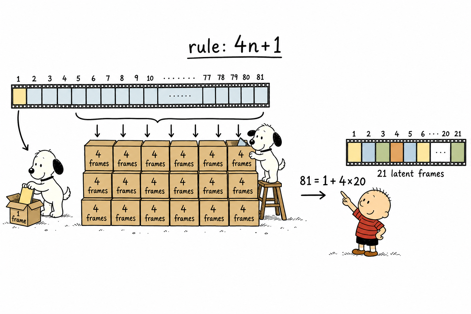
Why is the first frame special? Because the compression uses causal convolution. The first frame has no history before it to look at, so it can only stand alone as its own frame. This design also has a side effect: a static image can be treated as a video with F=1, which happens to occupy exactly one latent frame. Images and videos are therefore unified inside the same VAE representation, a point that will come up again in Chapter 7 when discussing image-to-video.
Causal Convolution and Streaming Inference
Look at the implementation of CausalConv3d in vae2_1.py; it is only a dozen or so lines:
class CausalConv3d(nn.Conv3d):

    def __init__(self, *args, **kwargs):
        super().__init__(*args, **kwargs)
        self._padding = (self.padding[2], self.padding[2], self.padding[1],
                         self.padding[1], 2 * self.padding[0], 0)
        self.padding = (0, 0, 0)

    def forward(self, x, cache_x=None):
        padding = list(self._padding)
        if cache_x is not None and self._padding[4] > 0:
            cache_x = cache_x.to(x.device)
            x = torch.cat([cache_x, x], dim=2)
            padding[4] -= cache_x.shape[2]
        x = F.pad(x, padding)
        return super().forward(x)
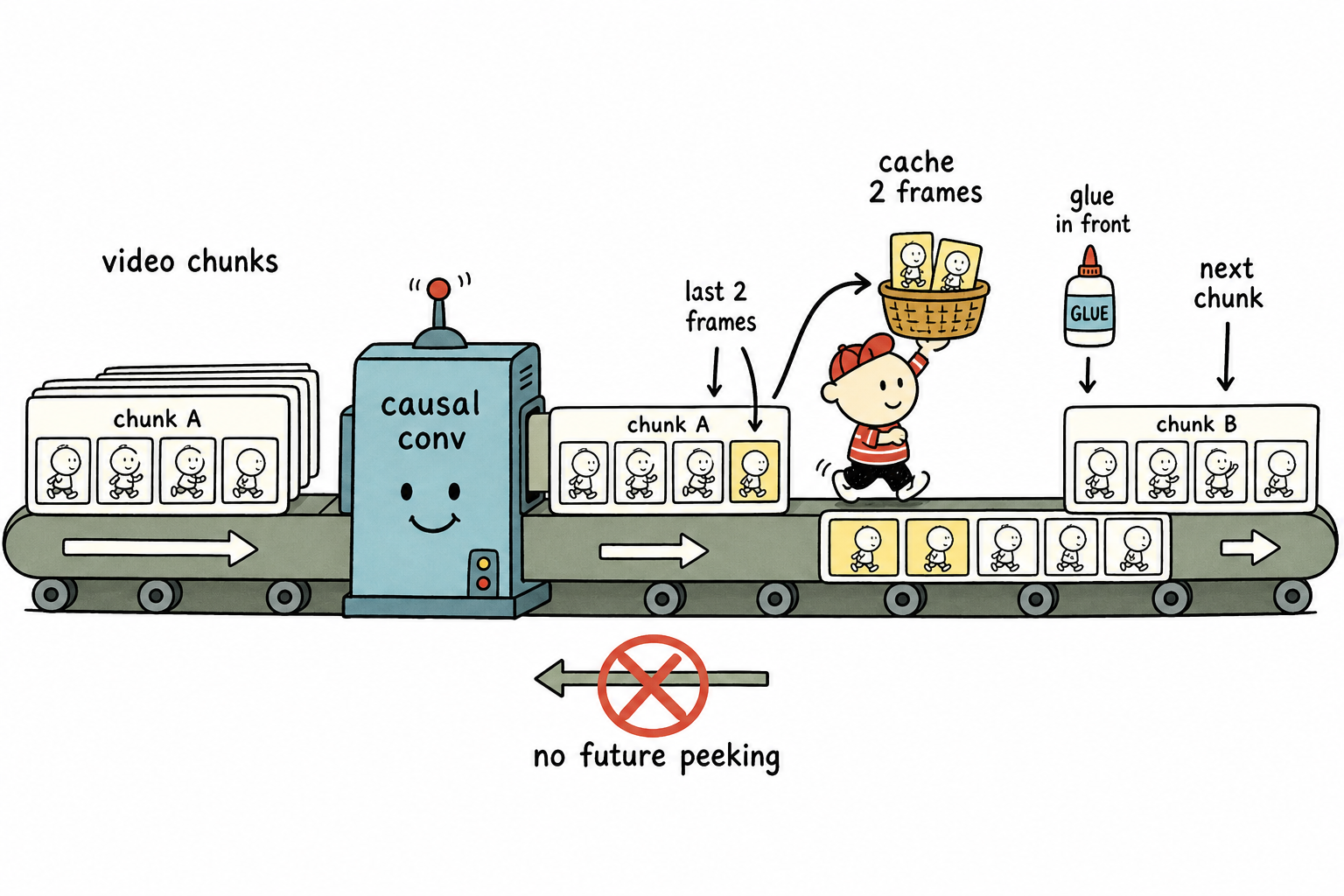
A regular 3D convolution pads symmetrically before and after the time dimension, so the output for each frame can “see” future frames. Here, all time padding is moved to the front, so each frame’s output depends only on the current frame and the past. There is one PyTorch detail worth knowing before reading this code: the arguments to F.pad are counted from the last dimension backward. The first four numbers handle width and height, and only the final pair (2 * self.padding[0], 0) belongs to the time dimension—double padding in front, zero padding behind.
Causality buys streaming processing: the video can be split into small chunks and passed through the network one by one. After each chunk is processed, the last 2 frames (CACHE_T = 2 at the top of the source file) are cached and prepended as cache_x for the next chunk, which is mathematically equivalent to convolving the whole video at once. As a result, the VAE’s memory usage is decoupled from the total video length. For this VAE stage, a 5-second video and a 50-second video have the same peak VRAM usage. The line padding[4] -= cache_x.shape[2] inside forward is just doing the accounting: however much zero padding the cache replaces, padding is reduced by the same amount.
The network itself is a standard hierarchical convolutional autoencoder, from the same family as Stable Diffusion’s VAE: three rounds of spatial downsampling correspond to 8× spatial compression, the latter two stages each halve the time axis to make 4× temporal compression, and the decoder climbs the same staircase back in reverse. Compared with the diffusion backbone, it is so small that it almost does not count in the budget—hundreds of millions of parameters versus 14B—but it determines the upper bound of generation quality. Details that the VAE cannot reconstruct cannot reach the pixel level no matter how well the diffusion model carves them out. Reconstruction quality, compression ratio, and decoding speed form a mutually exclusive triangle, and this is where video model teams quietly compete.
The “Exchange Rate” of Latent Space
The VAE and the diffusion model are two separately trained systems, and they connect through a hardcoded set of statistics. In vae2_1.py:
mean = [-0.7571, -0.7089, -0.9113, ..., -0.2921]   # per-channel means for 16 channels
std  = [ 2.8184,  1.4541,  2.3275, ...,  1.9160]   # per-channel standard deviations for 16 channels
self.scale = [self.mean, 1.0 / self.std]
These 32 numbers are computed from the training set. The raw output of VAE encode has very different scales across channels—the smallest std is 1.13 and the largest is 3.27, a threefold gap—while the diffusion model assumes it is dealing with data close to a standard normal distribution. So before latent enters the diffusion model, it must be standardized channel by channel; before decoding, it must be multiplied back. This set of numbers is the “exchange rate” between this pair of VAE and diffusion model. Swap in another VAE version, and all of it becomes invalid. The repository happens to contain another VAE used only by ti2v-5B: compression ratio 4×16×16, with 48 channels—the model being half the size is not enough; the data must shrink too. This is the key reason the 5B model can run 121 frames on a 24GB consumer GPU. The checkpoints of the two VAE versions are not interchangeable, and the root cause is this exchange rate. After being trained separately, the VAE is frozen; this Wan2.1 VAE version is directly reused by all four Wan2.2 tasks.
Chapter 3: Where Did the Prompt Go?
Every denoising step has to listen to the prompt, so the prompt first has to become something the model can compute.
Wan2.2 uses the encoder from umT5-XXL (Google’s multilingual T5 variant) to encode text: about 5.7B parameters, taking about 11.4GB in bf16—remember these two numbers; Chapter 6 will use them when calculating VRAM. The encoding call path is very short. In t5.py, T5EncoderModel.__call__ is straightforward:
def __call__(self, texts, device):
    ids, mask = self.tokenizer(
        texts, return_mask=True, add_special_tokens=True)
    ids = ids.to(device)
    mask = mask.to(device)
    seq_lens = mask.gt(0).sum(dim=1).long()
    context = self.model(ids, mask)
    return [u[:v] for u, v in zip(context, seq_lens)]
Tokenize, encode, then trim away padding for each item according to the real length from the attention mask. The prompt becomes a sequence of up to 512 vectors, each 4096-dimensional. This is the context. It has only one use inside the DiT: every layer’s cross-attention uses the video tokens as query, and the context as key/value. Text does not directly draw any pixels. Instead, during every denoising step, it continuously gives the model semantic direction—the prompt is not an order issued before work begins; it is the construction blueprint hanging on the wall for the entire job.
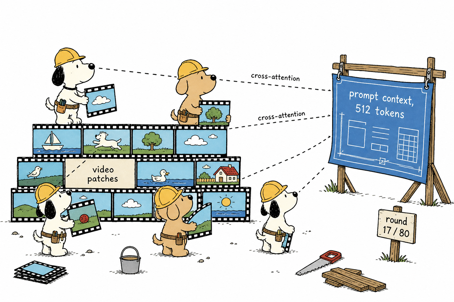
Why use T5 instead of the CLIP text tower commonly used in early text-to-image models? CLIP embeddings are good at “roughly what this sentence is about,” but the 77-token limit cannot fit detailed scene descriptions, and it is also weak on quantities and spatial relationships. T5 encodes token by token according to the structure of the text itself, supports up to 512 tokens, and works with token-level cross-attention, allowing the model to distinguish details like “the cat on the left is wearing red boxing gloves.” Choosing the multilingual umT5 has another consideration as well: Chinese prompts are first-class citizens. The official negative prompt is simply written in Chinese.
This refers to the negative prompt. The default value in the config is exactly:
wan_shared_cfg.sample_neg_prompt = '色调艳丽,过曝,静态,细节模糊不清,字幕,风格,作品,画作,画面,静止,整体发灰,最差质量,低质量,JPEG压缩残留,丑陋的,残缺的,多余的手指,画得不好的手部,画得不好的脸部,畸形的,毁容的,形态畸形的肢体,手指融合,静止不动的画面,杂乱的背景,三条腿,背景人很多,倒着走'
A checklist of “common failure scenes.” Its purpose will be discussed in Chapter 5 on CFG. For now, just remember: the negative prompt also goes through T5 and produces context_null.
One last prerequisite step: a prompt casually written by the user is often only one sentence, while the model was trained on long, detailed descriptions. Feeding it an overly short prompt reduces output quality. --use_prompt_extend first uses an LLM (DashScope online API or local Qwen2.5) to expand your prompt into a longer description with camera, lighting, action, and other details, then sends it to T5. In multi-GPU mode, expansion runs only once on rank 0 and is then broadcast to the other GPUs—LLM generation is random, so if 8 GPUs each expanded the prompt independently, you would get 8 different prompts, and the video could no longer be stitched together.
Chapter 4 DiT: Attention Over 75,600 Tokens
The pieces are in place: data lives in latent space (Chapter 2), text has become context (Chapter 3), and the learning target is the velocity field (Chapter 1). Now let’s look at the machine that predicts velocity: this is where all 14B parameters sit.
Before entering the backbone, it is worth answering a more fundamental question: what is the essential difference between a video model and an image model?
The answer is not as simple as “it has one more dimension.” If you call an image model frame by frame to generate 81 images, each frame may look beautiful on its own, but playing them together becomes a disaster: object shapes drift from frame to frame, lighting jumps, backgrounds shimmer. In the jargon, this is called flicker. Temporal consistency has to be modeled explicitly. The industry has explored two paths: factorized attention (spatial attention and temporal attention are done separately: first make each frame internally coherent, then align along the time axis; cheaper, but with a ceiling on consistency) and full 3D joint attention (all patches from all frames are placed into the same attention operation, so any token can directly see any position at any moment; strongest consistency, but sequence length explodes). Wan2.2 takes the second path, and that choice directly leads to the protagonist of this chapter: a sequence of 75,600 tokens.
From Latent to Token
Before the latent enters the DiT, it is first split into patches. This step is called patchify. In model.py, it is simply a Conv3d whose stride equals its kernel size:
self.patch_embedding = nn.Conv3d(
    in_dim, dim, kernel_size=patch_size, stride=patch_size)
patch_size = (1, 2, 2): the time dimension is not split, while every 2×2 spatial block in the latent is convolved into a 5120-dimensional token. Counting the total:
Tokens per latent frame = 90 × 160 / (2×2) = 3600
Total tokens            = 3600 × 21 frames = 75600
75,600 is the self-attention sequence length when generating a 5-second 720p video. SDXL generating a 1024 image has a sequence length of 4096; video is 18 times longer than image. Attention compute grows with the square of sequence length, so 18× length means about 340× attention cost. All the VRAM issues and sequence parallelism discussed later ultimately originate from this number.
How 14B Is Counted
The config gives dim=5120, ffn_dim=13824, num_layers=40. The parameter bulk in each layer is:
self-attention:  four Q/K/V/O matrices = 4 × 5120² ≈ 105M
cross-attention: same four matrices    = 4 × 5120² ≈ 105M
FFN:             two matrices          = 2 × 5120 × 13824 ≈ 142M
Per layer total ≈ 351M, × 40 layers ≈ 14.05B
That is where the 14B in “A14B” comes from; embeddings and modulation parameters are only a rounding error. bf16 uses 2 bytes per parameter, so one expert is 28GB. t2v-A14B has two experts (Chapter 6 explains why), meaning the DiT weights alone take 56GB. Add T5’s 11.4GB, the VAE, and activations during sampling, and this is how the 80GB single-GPU threshold gets filled.
The Full Forward Pass of One Block
WanAttentionBlock.forward is the smallest repeating unit of the whole model, and it is worth reading line by line. Before reading it, one reminder: the parameter e comes from timestep t—the tick mark on the ruler from Chapter 1, where 999 is almost pure noise and 0 is the finished video. How it becomes e will be explained right after the code.
def forward(self, x, e, seq_lens, grid_sizes, freqs, context, context_lens):
    assert e.dtype == torch.float32
    with torch.amp.autocast('cuda', dtype=torch.float32):
        e = (self.modulation.unsqueeze(0) + e).chunk(6, dim=2)
    assert e[0].dtype == torch.float32

    # self-attention
    y = self.self_attn(
        self.norm1(x).float() * (1 + e[1].squeeze(2)) + e[0].squeeze(2),
        seq_lens, grid_sizes, freqs)
    with torch.amp.autocast('cuda', dtype=torch.float32):
        x = x + y * e[2].squeeze(2)

    # cross-attention & ffn function
    def cross_attn_ffn(x, context, context_lens, e):
        x = x + self.cross_attn(self.norm3(x), context, context_lens)
        y = self.ffn(
            self.norm2(x).float() * (1 + e[4].squeeze(2)) + e[3].squeeze(2))
        with torch.amp.autocast('cuda', dtype=torch.float32):
            x = x + y * e[5].squeeze(2)
        return x

    x = cross_attn_ffn(x, context, context_lens, e)
    return x
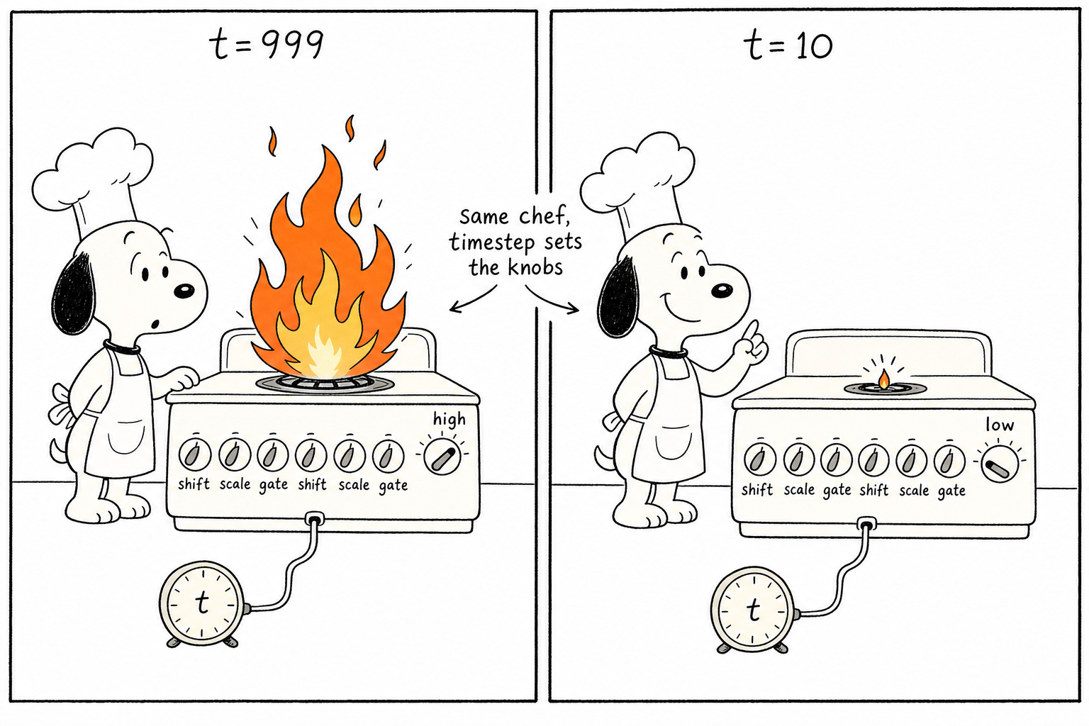
There are three sections: Self-Attention (75,600 tokens looking at one another to establish spatiotemporal consistency), Cross-Attention (looking at the text context to inject semantics), and FFN. The truly interesting part is e, which is chunked into 6 pieces:
| Used where | Role | |
|---|---|---|
| e[0], e[1] | before self-attn norm | shift and scale, norm(x) * (1+scale) + shift |
| e[2] | self-attn output | gate, controls how much this branch adds into the residual |
| e[3], e[4] | before FFN norm | same shift/scale as above |
| e[5] | FFN output | gate |
Where do these 6 groups of parameters come from? The scalar t (for example, 927) first goes through a standard sinusoidal embedding and expands to 256 dimensions—the network has poor resolution over a single scalar, so after expansion, high-frequency channels handle fine granularity while low-frequency channels handle coarse granularity—then it passes through an MLP and a projection:
self.time_embedding = nn.Sequential(
    nn.Linear(freq_dim, dim), nn.SiLU(), nn.Linear(dim, dim))
self.time_projection = nn.Sequential(nn.SiLU(), nn.Linear(dim, dim * 6))
dim * 6 corresponds exactly to those 6 modulation chunks. This technique is called AdaLN (adaptive layer norm), one of the core contributions of the DiT paper: instead of concatenating t into the sequence as a token, t modulates the scale, shift, and residual gates of each layer’s normalization. Intuitively, return to the denoising trajectory from Chapter 1: when t=999, the input is almost pure noise, so the network should make bold strokes; when t=10, the image is basically formed, so the network should only make small refinements. The same set of weights switches behavior modes through these 6 groups of parameters that vary with t, like the same chef automatically changing heat levels according to how close the dish is to completion. The DiT paper compared two schemes—“concatenate t as a token” versus “AdaLN modulation”—and the latter achieved significantly better FID under the same compute. It has since become the default design for diffusion transformers.
There is another easily missed detail in the code: all modulation operations are wrapped in autocast float32. The backbone can run in bf16, but these modulation steps are forced to full precision. Denoising is an iterative process over dozens of steps, and numerical error in the modulation parameters can accumulate gradually. This is where the authors spend VRAM in exchange for stability.
3D RoPE: Letting Tokens Know Where They Are
The 75,600 tokens are arranged into a one-dimensional sequence, and attention itself does not know who is next to whom. Positional information is injected by RoPE (rotary position embedding). The special part in the video version is that coordinates have three axes. During construction, each head’s 128 dimensions are split into three sections:
d = dim // num_heads          # 5120 // 40 = 128
self.freqs = torch.cat([
    rope_params(1024, d - 4 * (d // 6)),   # time axis: 44 dims
    rope_params(1024, 2 * (d // 6)),       # height axis: 42 dims
    rope_params(1024, 2 * (d // 6))        # width axis: 42 dims
], dim=1)
When applied, each token takes three segments of rotation values according to its own (f, h, w) coordinates, concatenates them into a complete 128-dimensional rotation, and applies it to q and k in one step using complex multiplication. When attention computes the q·k inner product, the relativity of rotation makes the inner product depend only on the coordinate difference between the two tokens: shift the entire image by two cells, and all relative relationships remain unchanged, so the patterns learned by the model still apply. Translation invariance comes for free. This is a direct extension of image 2D RoPE to video. The 44/42/42 allocation means the time axis receives roughly the same number of frequency channels as a single spatial axis, so temporal and spatial relationships are treated with comparable importance.
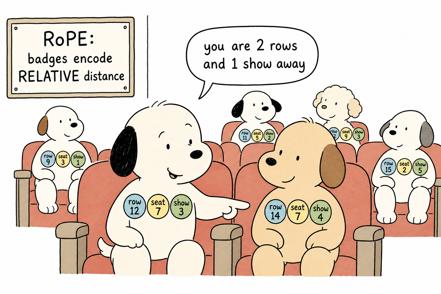
Detail: the rotation implementation (rope_apply) runs entirely in float64 and explicitly disables autocast. Rotation is a purely geometric operation; half-precision phase errors can be amplified on long sequences, so this is another tradeoff of spending compute for numerical stability. In addition, inside WanSelfAttention, after q and k pass through their linear layers, each is followed by an RMSNorm (QK-Norm) to clamp the scale of the inner products and prevent softmax saturation. Its value is not obvious from inference code, but without it, a 14B-scale DiT is very hard to train stably.
Shape bookkeeping for one forward pass
Putting the whole chapter into one table, here is every shape transformation from model input to model output (t2v-A14B, 81 frames, 720p, single GPU):
| Stage | Tensor Shape | Notes |
|---|---|---|
| Noisy latent | 16 × 21 × 90 × 160 | The space defined by the VAE in Chapter 2 |
patch_embedding (Conv3d) | 5120 × 21 × 45 × 80 | Spatial 2×2 patch is convolved into one position |
| Flattened into sequence | 75600 × 5120 | 21×45×80 = 75600 |
40 × WanAttentionBlock | 75600 × 5120 | Shape unchanged, content repeatedly refined; inside each layer, q/k/v are split into 40 heads × 128 dimensions, and RoPE rotates only q and k |
| Head | 75600 × 64 | 64 = patch volume (1×2×2) × 16 channels |
unpatchify | 16 × 21 × 90 × 160 | Folded back into the latent shape |
Whatever shape goes in is the shape that comes out; the middle consists of 40 equal-width refinement layers. The semantics of the output are the velocity from Chapter 1, corresponding point-by-point to the input latent: the value at each position indicates “which direction the content at this position should move.” The text context (512 × 4096 projected by text_embedding to 512 × 5120) exists throughout only as the key/value for cross-attention and does not occupy sequence positions.
At this point, the machine that “takes a noisy latent and a t, then outputs a velocity prediction” is complete. The next chapter looks at how this prediction is used by the sampling loop.
Chapter 5 Sampling Loop: 40 Steps, Two Forward Passes per Step
The machine only reports a direction each time; what really walks the video out of noise is the loop around it: choose 40 stops, and ask for directions twice at each stop.
UniPC: How to Move Fast and Steadily
Once we have the velocity field, we still need a numerical integrator: at each step, take the velocity reported by the model and decide how far to move forward. This component is called the scheduler in code, and fm_solvers_unipc.py is exactly that. The simplest integration is Euler’s method: assume the velocity is constant at each step, x ← x - Δσ·v. It is first-order accurate. But the real velocity field is curved, so the larger the step, the farther it drifts. Wan2.2’s default UniPC is a multistep predictor-corrector: the predictor uses the model outputs from the most recent two steps, configured as solver_order=2, to fit the trend of velocity change and extrapolate to the next step; after the model output at the new position is computed, the corrector goes back and revises the step just taken, gaining another order of accuracy for free without spending an extra forward pass. With the same 40 model calls, the local error drops from Euler’s first-order small term to third order. This is how the step budget for “acceptable quality” gets cut from hundreds to dozens—video generation needs two 14B forward passes per step, so every saved step is real money.
shift: Where the 40 Stops Land
The scheduler is also responsible for deciding where the 40 sampling points are placed. set_timesteps first lays points out uniformly, then applies the shift transform:
sigmas = shift * sigmas / (1 + (shift - 1) * sigmas)
This transform squeezes the points toward the high-noise end, where σ is large. How much does it squeeze? Look at the median:
| shift | median timestep |
|---|---|
| 1 (no squeeze) | 512 |
| 5 | 840 |
| 12 (t2v default) | 926 |
When shift=12, half of the sampling points fall in the t>926 interval. The actual timestep sequence starts like this, with shift=12 and 40 steps; you can verify it yourself by running set_timesteps, with the output rounded to integers:
999, 997, 995, 993, 990, 988, ...
The first few steps are spaced only about 2 apart, so the loop walks extremely densely; by the low-noise stage, the spacing stretches to dozens, and it crosses the stage in just a few steps.
Why allocate it this way? The high-noise stage determines composition, objects, and motion direction—the “from nothing to something” phase. The low-noise stage mostly polishes details. Tilting the budget toward the harder phase is a tradeoff video generation needs more than image generation does: image models usually use a shift of around 3, but motion consistency in video is much harder, so Wan2.2 raises it directly to 12. In the same repository, i2v uses 5.0 because the first frame is already given and the structural pressure is lower; ti2v-5B uses 5.0; s2v uses 3. Each task’s shift tells its own difficulty distribution. --sample_shift does not change the number of steps, only how those steps are allocated. Tuning it means moving budget between “more stable structure” and “finer details”—and it also meshes tightly with the expert split in the next chapter. We will do the numerical accounting there.
CFG: Why Each Step Runs Two Forward Passes
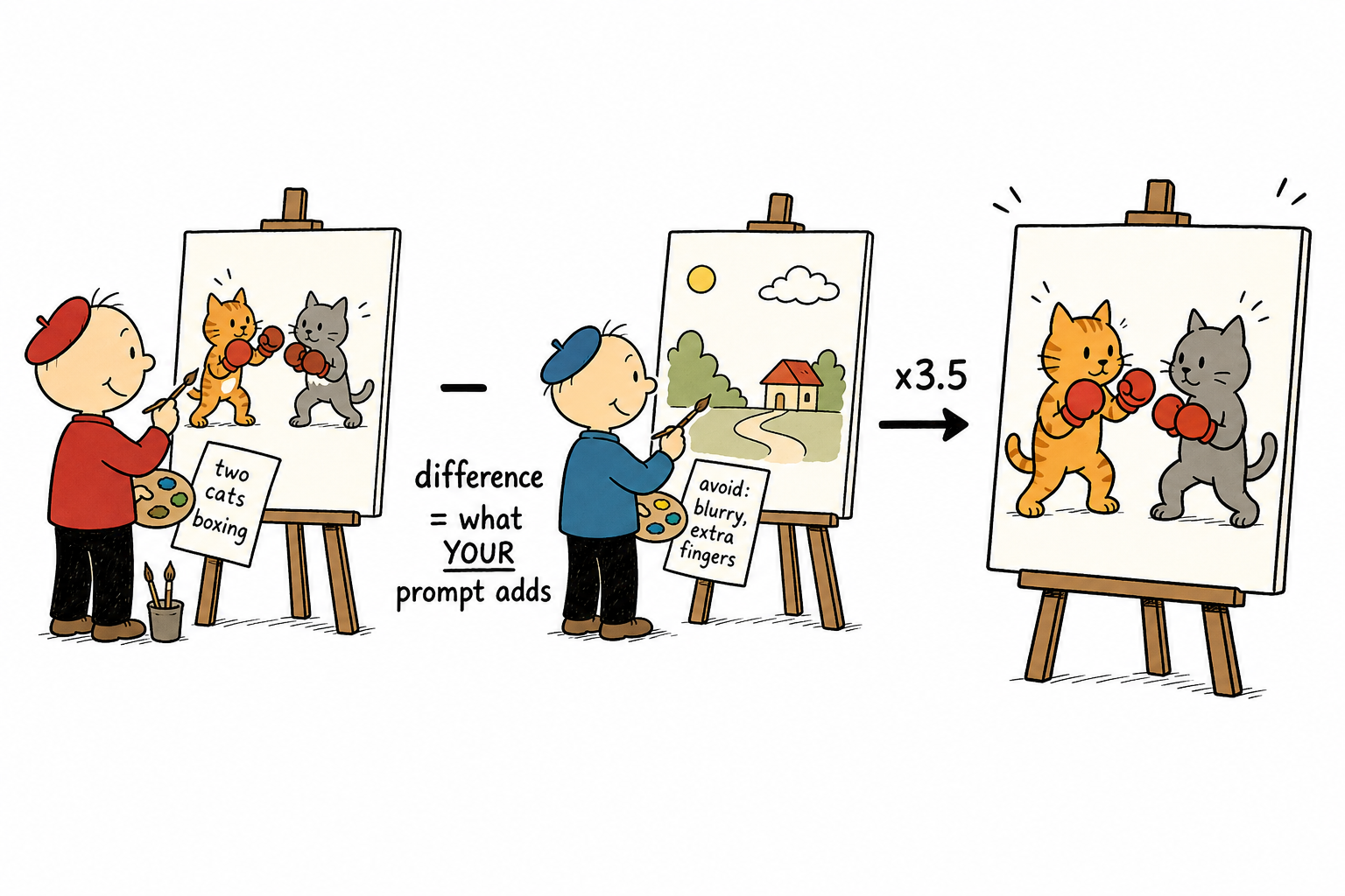
The core of the sampling loop, in text2video.py:
noise_pred_cond = model(latent_model_input, t=timestep, **arg_c)[0]
noise_pred_uncond = model(latent_model_input, t=timestep, **arg_null)[0]

noise_pred = noise_pred_uncond + sample_guide_scale * (
    noise_pred_cond - noise_pred_uncond)
For the same latent and the same t, it runs twice: once with your prompt, where arg_c contains context, and once with the negative prompt, where arg_null contains context_null. This is classifier-free guidance (CFG).
The principle deserves one layer of math. To generate samples that satisfy condition c, decompose it with Bayes’ rule:
p(x|c) ∝ p(x) · p(c|x)
Take the log and then the gradient, the score:
∇log p(x|c) = ∇log p(x) + ∇log p(c|x)
The first term is the unconditional direction, what the data itself looks like. The second term is the classifier gradient that “makes x look more like it belongs to condition c.” Early methods really trained a separate classifier to provide it, which was expensive and hard to train. CFG’s insight is that this term can be obtained for free: the model has learned both conditional and unconditional predictions, by randomly dropping text during training, so subtracting the two gives:
∇log p(c|x) = ∇log p(x|c) - ∇log p(x) ≈ conditional prediction - unconditional prediction
The classifier gradient is hidden in the difference between the two forward passes. During sampling, amplify this term by w:
final direction = uncond + w · (cond - uncond)
Compare this with the three lines of code above: it is exactly the same. sample_guide_scale is w.
Choosing w is a pure tradeoff. w=1 degenerates into conditional generation: the image looks natural, but often “doesn’t understand” the prompt. Raise w, and the model is strongly pushed toward regions where the “classifier” is more confident; composition obedience improves, at the cost of oversaturated colors, mushy details, and stiff motion, because the latent is pushed away from the high-density region of the training distribution. Image models often use around 7. Video is more sensitive to temporal naturalness, so Wan2.2’s A14B dual-expert series only uses 3.0–4.0; ti2v-5B uses 5.0, and s2v uses 4.5.
The role of the negative prompt in this derivation is also clear: standard CFG uses empty text for uncond; Wan2.2 replaces it with that string describing “overexposure, deformation, three legs,” and so on. The difference direction changes from “move closer to your prompt” into “move closer to your prompt while moving away from these defects.” One forward pass does two jobs at once.
The cost is just as clear: 40 steps × 2 forward passes = 80 full inferences through the 14B model. Video generation is slow, and half the bill is charged to CFG.
Chapter 6: Two 14B Experts Taking Turns
The denoising loop and CFG in the previous chapter assume that one model is running behind the scenes. In fact, the A14B series hides two. This chapter explains how they divide the work, and why that directly determines whether your GPU has enough memory.
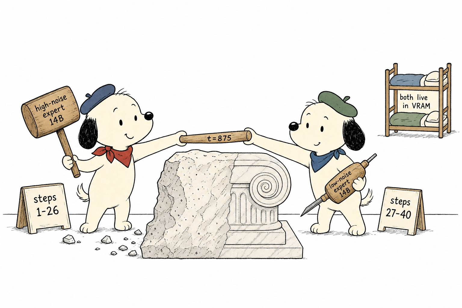
The signature design of the Wan2.2 A14B series is that two 14B experts handle different noise ranges. In the config:
t2v_A14B.boundary = 0.875
t2v_A14B.sample_guide_scale = (3.0, 4.0)  # low noise, high noise
At each step, the sampling loop checks t >= 0.875 × 1000: if true, it uses high_noise_model; otherwise it uses low_noise_model. The motivation follows from the observation in Chapter 5: the high-noise stage determines structure out of chaos, while the low-noise stage polishes textures on a semi-finished result. Instead of forcing one network to master both jobs, it is better to let two networks each specialize in one. And this division already holds from the very first layer: the high-noise expert receives something close to pure Gaussian noise, so its early layers are “guessing structure from statistics”; the low-noise expert receives a semi-finished image, so its early layers are “reading the existing picture.” The input distributions are so different that sharing the lower layers would only drag both sides down. So the two experts are fully independent, trained separately on their own noise ranges, and take turns at inference time according to t.
This is what the official “27B total parameters, 14B active” means: 27B is the precise count, while the 14.05B from Chapter 4 only counted the major parts of each layer. Capacity doubles, but only one expert runs at any given step, so the compute cost is equivalent to a dense 14B model. Don’t be misled by the word “MoE”: LLM MoEs like Mixtral choose experts per layer and per token using a learned router. Here, routing happens at the timestep level, the threshold is hard-coded, there is no router at all, and the whole implementation is just an if. This coarse granularity brings two benefits: diffusion timesteps are already natural difficulty labels, so there is no need to train a router; and the two experts can be trained and upgraded independently.
Here is the full sampling loop. All the parts discussed in previous chapters come together in these 20 lines:
for _, t in enumerate(tqdm(timesteps)):
    latent_model_input = latents
    timestep = [t]

    timestep = torch.stack(timestep)

    model = self._prepare_model_for_timestep(
        t, boundary, offload_model)
    sample_guide_scale = guide_scale[1] if t.item(
    ) >= boundary else guide_scale[0]

    noise_pred_cond = model(
        latent_model_input, t=timestep, **arg_c)[0]
    noise_pred_uncond = model(
        latent_model_input, t=timestep, **arg_null)[0]

    noise_pred = noise_pred_uncond + sample_guide_scale * (
        noise_pred_cond - noise_pred_uncond)

    temp_x0 = sample_scheduler.step(
        noise_pred.unsqueeze(0), t,
        latents[0].unsqueeze(0),
        return_dict=False, generator=seed_g)[0]
    latents = [temp_x0.squeeze(0)]
Each round does five things: choose the expert, choose the guide scale, run two forward passes, combine them with CFG, and let the scheduler take one step. _prepare_model_for_timestep also contains the single-GPU lifesaving offload logic:
if offload_model or self.init_on_cpu:
    if next(getattr(self, offload_model_name).parameters()).device.type == 'cuda':
        getattr(self, offload_model_name).to('cpu')
    if next(getattr(self, required_model_name).parameters()).device.type == 'cpu':
        getattr(self, required_model_name).to(self.device)
With --offload_model True enabled, each time the expert switches, the off-duty one is moved back to system memory and the on-duty one is moved onto the GPU. Moving 28GB of weights across PCIe takes several seconds, but fortunately the whole sampling process switches only once: t decreases monotonically, and once it crosses the boundary, it never goes back. So this cost is paid only once.
How boundary and shift Interact
This is the easiest piece of accounting to miss when tuning. boundary=0.875 looks, literally, like “only 12.5% of timesteps belong to the high-noise expert.” But as Chapter 5 explained, shift aggressively squeezes the sampling points toward the high-noise end. Counting the 40 steps where t ≥ 875 gives:
| shift | High-noise expert steps (t ≥ 875) |
|---|---|
| 1 | 5 / 40 |
| 5 | 17 / 40 |
12 (t2v default) | 26 / 40, or 65% |
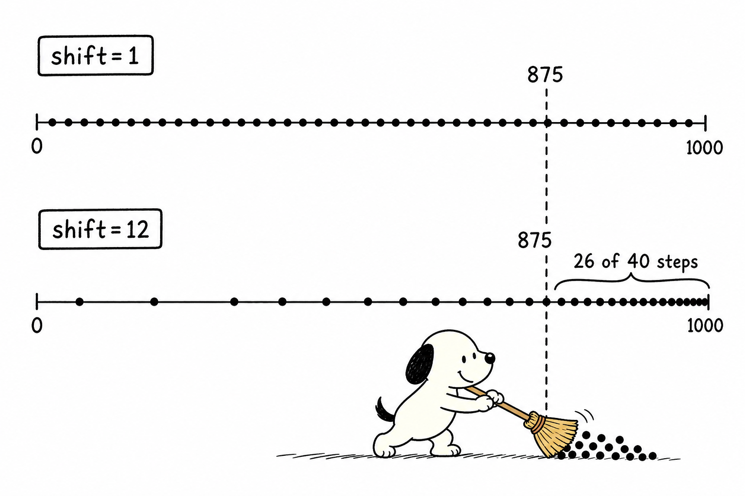
Most of the budget goes to the high-noise expert that determines structure, while the low-noise expert uses the remaining 14 steps to finish things off. If you tune --sample_shift alone without changing boundary, the workload split between the two experts changes silently, and the resulting quality fluctuations can be hard to reason about. The two guide_scale values also serve this division of labor: the high-noise stage uses 4.0 to stay close to the prompt during structure formation, while the low-noise stage drops to 3.0 so the detail stage is pushed less aggressively and the image looks more natural.
Finally, let’s clear up a common misunderstanding: only one expert appears at each timestep. The two forward passes are the CFG cond and uncond passes; the experts never work simultaneously in the same step. “Two forward passes per step” and “two experts” are orthogonal things.
VRAM Accounting and the Three-Piece Kit
Run the numbers again: two experts in bf16 weights take 56GB, the T5 encoder takes 11.4GB, plus the VAE, activations, KV cache, and other overhead. An 80GB card can just barely fit everything. When a single card cannot handle it, the three-piece kit targets specific items on the bill: --offload_model True moves the currently unused expert back to system memory, removing 28GB of resident VRAM; --t5_cpu keeps T5 in system memory and only moves it onto the GPU during encoding, saving 11.4GB; --convert_model_dtype lowers weight precision.
How should you combine them? The README’s example commands give the official answer: the single-GPU A14B example already includes --offload_model True --convert_model_dtype and notes that at least 80GB of VRAM is required. For running ti2v-5B on a 4090, all three are added, including --t5_cpu; in the 5B scenario, T5’s 11.4GB becomes proportionally the biggest item. The README’s ti2v-5B section also gives the reverse hint: if VRAM exceeds 80GB, remove these flags for a clear speedup, because offloading is not free.
Chapter 7 Conditional Injection: Which Lines Changed for Image-to-Video
By this point, you’ve already walked through the complete text-to-video pipeline. The remaining four tasks—image-to-video, text-image unified generation, audio, and animation—are not four brand-new model families. They are different “prompts” swapped onto the same backbone.
There are only three ways to add conditions:
- cross-attention: the path used by text, where the condition is attended to as key/value
- channel concatenation: the condition tensor is directly concatenated with the noise latent along the channel dimension, then fed into patch embedding together
- AdaLN: the condition is mixed into the timestep embedding to modulate each layer’s norm
Image-to-video (i2v-A14B) uses the second method. Look at how image2video.py constructs the condition:
msk = torch.ones(1, F, lat_h, lat_w, device=self.device)
msk[:, 1:] = 0
msk = torch.concat([
    torch.repeat_interleave(msk[:, 0:1], repeats=4, dim=1), msk[:, 1:]
], dim=1)
msk = msk.view(1, msk.shape[1] // 4, 4, lat_h, lat_w)
msk = msk.transpose(1, 2)[0]
...
y = torch.concat([msk, y])
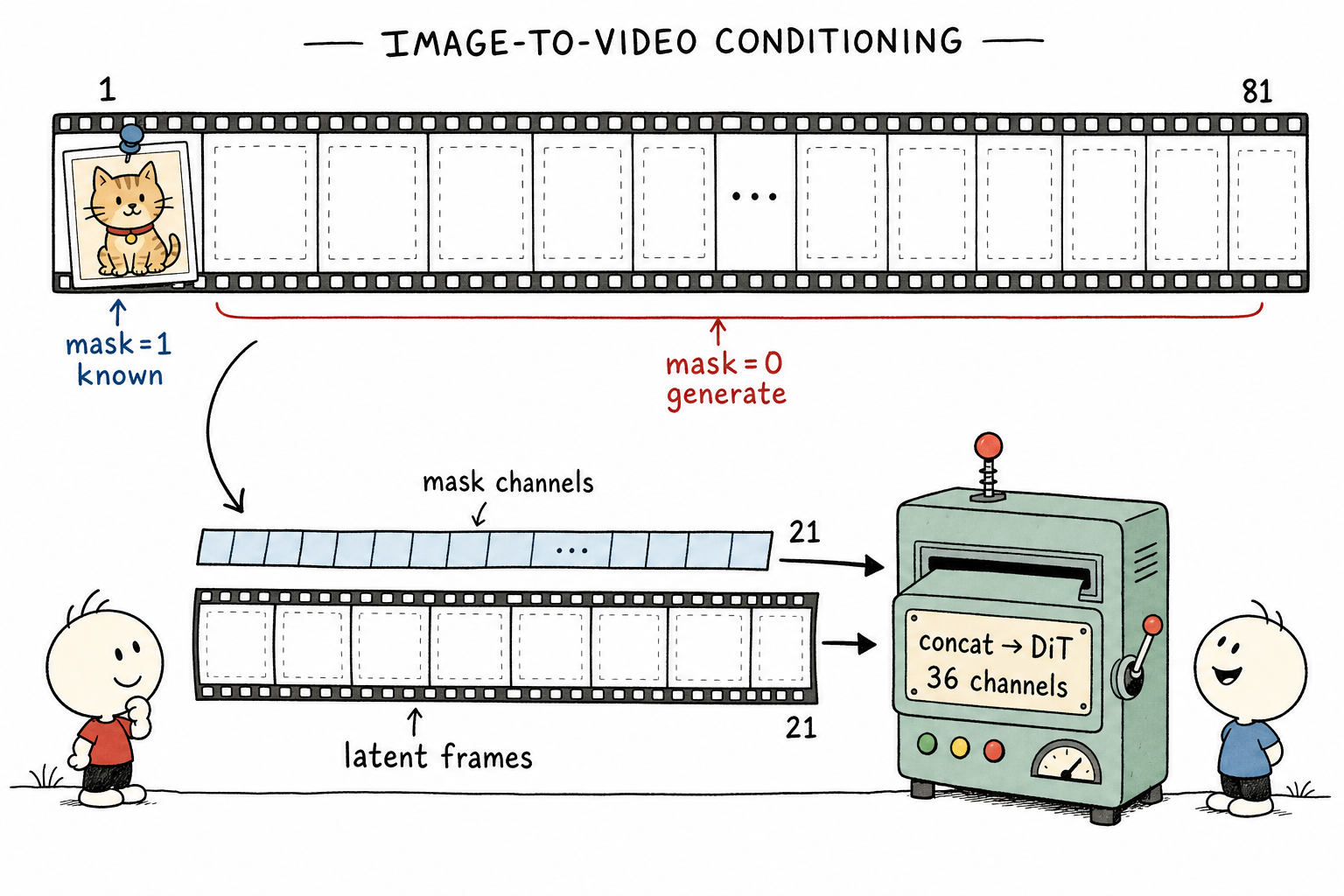
Line by line: msk is the marker for “which frames are known.” The first frame—the input image—is marked as 1, and the remaining 80 frames are marked as 0. The following repeat_interleave plus reshape sequence does one thing: it folds the 81-frame pixel-level mask onto the 21-frame latent timeline. Remember the VAE compression rule from Chapter 2? The first frame gets its own latent frame, and every 4 frames after that are merged into one. The mask has to be folded by the same rule: copy the first frame 4 times to complete the grouping, then fold every 4 frames into one group, yielding a 4×21×h×w mask aligned with the latent.
y is the input image itself after passing through the VAE encoder, with the missing frames padded by zeros. The mask and y are concatenated into 20 channels, then concatenated once more with the 16-channel noise latent along the channel dimension before entering the model. At the start of forward in model.py:
if y is not None:
    x = [torch.cat([u, v], dim=0) for u, v in zip(x, y)]
The i2v version of WanModel has 36 input channels: 16 noise channels + 16 image latent channels + 4 mask channels. The first convolution in patch embedding is wider than in the t2v version, while the remaining 40 layers have exactly the same structure. The entire backbone change for image-to-video is simply that the input channels go from 16 to 36.
What the model learns from these 36 channels is: copy the given content where mask=1, generate where mask=0, and keep the two spatially and temporally coherent. The first frame pins down the subject and style of the image, while the next 80 frames unfold motion around it. That is the mechanism behind “making an image move.”
Where the Conditions Come From in Other Tasks
Read the other three tasks with the same mindset. Focus on: “What is the condition, and through which entrance does it enter the model?”
ti2v-5B (unified text-image generation). The same 5B backbone is paired with a high-compression 4×16×16 VAE, supporting both t2v and i2v without changing the architecture. If an image is provided, it is encoded, pinned into the first latent-frame position, and marked as known with a mask. If no image is provided, generation starts from pure noise. One model, two faces.
s2v-14B (audio-driven generation). The condition is audio: wav2vec2 turns the waveform into frame-level features, which are re-bucketed and aligned to the video frame rate before being injected into the model, driving lip motion and body rhythm. The video length follows the audio length. Extra-long audio is split into multiple segments and generated autoregressively, with each segment using the last few latent frames from the previous segment as a “momentum condition” for continuity. This is the only long-video solution in the repository.
animate-14B (character animation/replacement). This is the most condition-heavy task: a skeletal pose sequence drives motion, a facial feature sequence drives expressions, the reference image goes through CLIP visual encoding and enters cross-attention to lock identity, and in replacement mode there is also a background video and mask. Multiple condition streams enter through their own separate openings.
The condition sources vary wildly, but the injection methods are always permutations of the same three ideas: channel concatenation for spatially aligned conditions such as masks, poses, and backgrounds; cross-attention for global semantic conditions such as text and reference-image features; and frame-level feature injection for temporally aligned conditions such as audio. Once you understand one task, the rest are just combinations.
Chapter 8: What Does 75600² Actually Mean?
We have finished explaining how the model works and how conditions are injected. What remains is a pure engineering problem: with this much computation, what do you do when a single GPU cannot handle it? This chapter returns to the 75600 from Chapter 4 and looks at how it forces a multi-GPU solution.
Let’s calculate the attention bill in detail. The core computation of a single self-attention layer is two matrix multiplications, QK^T and AV. The FLOPs are approximately:
2 × 2 × L² × dim = 4 × 75600² × 5120 ≈ 1.17 × 10¹⁴
(The two 2s mean: one for the two matrix multiplications, and one because each multiply-add pair counts as two FLOPs.) One layer is 117 TFLOPs. Across 40 layers and 80 forward passes, attention alone reaches the order of 3.7 × 10¹⁷ FLOPs. An A100 has a bf16 peak throughput of about 312 TFLOPS, so even under ideal utilization this part alone would take around twenty minutes, without counting the FFN. This is the physical baseline behind “a 5-second video takes minutes to tens of minutes to generate.”
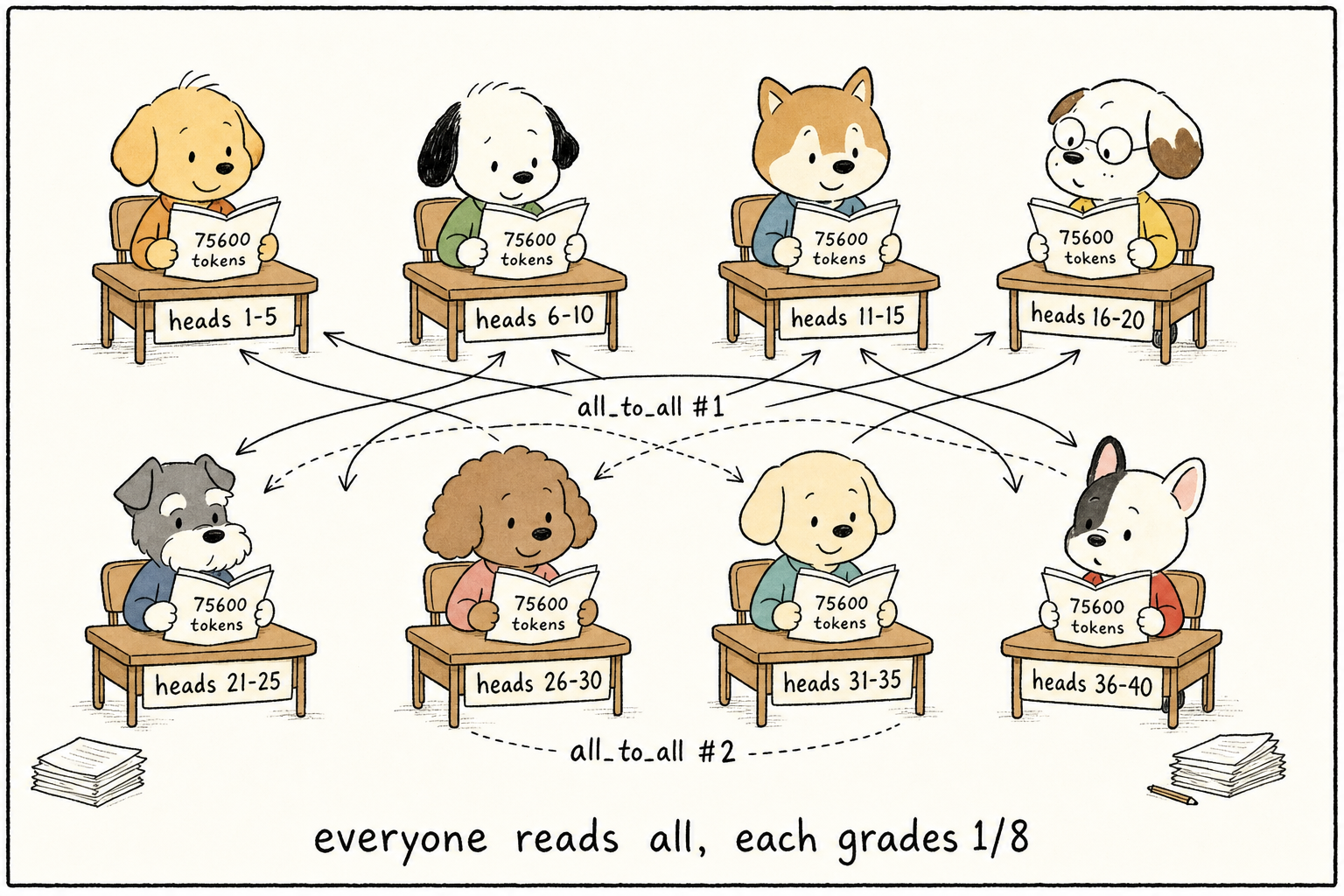
If one GPU cannot handle it, split it. Wan2.2’s main solution is Ulysses sequence parallelism. The core communication primitive lives in distributed/util.py: a dimension exchange.
def all_to_all(x, scatter_dim, gather_dim, group=None, **kwargs):
    world_size = get_world_size()
    if world_size > 1:
        inputs = [u.contiguous() for u in x.chunk(world_size, dim=scatter_dim)]
        outputs = [torch.empty_like(u) for u in inputs]
        dist.all_to_all(outputs, inputs, group=group, **kwargs)
        x = torch.cat(outputs, dim=gather_dim).contiguous()
    return x
Attention requires every token to see the full sequence, so you cannot simply split the sequence and call it done. Ulysses’ answer is: “split heads, not the sequence.” On 8 GPUs, tracing the tensor shapes through one pass gives the following (B=1, L=75600, 40 heads):
| Stage | Held by each GPU |
|---|---|
| Before entering the block, sequence is split | L=9450, 40 heads |
all_to_all scatter head dimension, gather sequence dimension | L=75600, 5 heads |
| Local flash attention | Full sequence, 1/8 of heads |
all_to_all back | L=9450, 40 heads |
Two rounds of communication reduce both attention computation and activation memory per GPU to 1/8, because each GPU only computes 1/8 of the attention heads. The number of heads must be divisible by the number of GPUs; 40 heads with 8 GPUs fits perfectly. generate.py contains the corresponding assert.
There is also a sequence-length detail prepared specifically for multi-GPU execution. In text2video.py, the tail of the seq_len formula includes a pair of ceil(... / sp_size) * sp_size, rounding the token count up to an integer multiple of the GPU count. 75600 happens to be divisible by 8, so it remains unchanged. If another resolution produces 75601 tokens, it is padded to 75608, ensuring that each GPU receives an equal-length slice. On a single GPU, sp_size=1, so this expression is an identity; it only reveals its purpose in the multi-GPU setting.
The communication cost can also be calculated: per layer, q/k/v/output require four all_to_all calls, totaling about 3.1 GB of data. Across 40 layers and 80 forward passes, that accumulates to about 10 TB. That sounds scary, but NVLink inter-GPU bandwidth is on the order of hundreds of GB per second, so spread across the whole generation process, communication time is much smaller than compute time. The trade is worthwhile. On PCIe machines, however, this may not hold; multi-GPU speedup will shrink noticeably. As a side note, the competing approach Ring Attention splits the sequence and circulates K/V around the ring. It is not constrained by divisibility of head count, but its communication is more complex. Ulysses is capped by the number of heads: the GPU count cannot exceed 40 heads, so a 64-GPU cluster needs another scheme.
Parameters not fitting is another axis: FSDP (fully sharded data parallel) splits model weights into N shards and places them across GPUs. During the forward pass, when execution reaches a given layer, all GPUs first all-gather that layer’s parameters, compute the layer, then immediately release them. With 8 GPUs, the resident DiT weights per GPU drop from 56 GB to 7 GB. The cost is one all-gather per layer, but on NVLink most of this overhead can be overlapped with computation.
Putting the single-GPU and 8-GPU memory accounts side by side:
| Item | Single GPU without offload | 8 GPUs fsdp + ulysses |
|---|---|---|
| Two DiT expert weights bf16 | 56 GB | 7 GB / GPU |
| T5 encoder weights | 11.4 GB | Sharded or close to 0 after --t5_cpu |
| Attention activations | Full sequence | 1/8 sequence |
| Conclusion | 80GB GPU is near the edge | Midrange GPUs are enough |
Sequence parallelism handles compute; FSDP handles memory. They are orthogonal, so --dit_fsdp --ulysses_size 8 can be enabled at the same time. The 8-GPU command in the README includes both of them for a reason: every flag corresponds to a line in the accounting.
Chapter 9: Why the Model Makes the Mistakes It Often Makes
Most typical video-generation failures can be traced back to the principles discussed earlier. This chapter connects the “symptoms” to the “mechanisms,” which is more useful than memorizing a checklist.
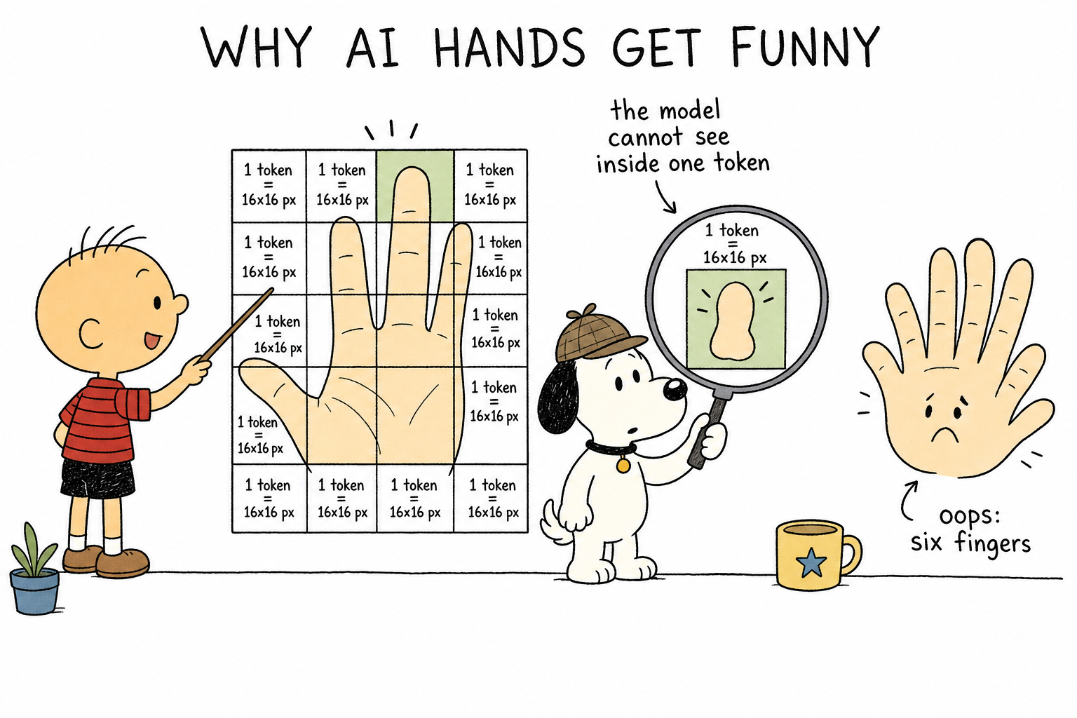
Broken fingers, text, and fine structures. This is the result of two levels of compression working together. The VAE compresses an 8×8 pixel block into one latent position, and patchify then merges 2×2 latents into one token, so one token governs 16×16 pixels. A finger is often only a dozen or so pixels wide; an entire finger may fall into one or two tokens. No matter how strong attention is, it cannot distinguish the boundaries of five fingers inside a token. Text is even worse, because strokes are pixel-level details. The only remedies are lowering the compression ratio or increasing resolution, both of which run directly into the compute wall. This is a structural weakness of the current generation of architectures, not the fault of the training data.
Drift in the later part of long videos. t2v generates 81 frames in one shot, with inter-frame consistency enforced by full 3D attention, so it works fine within 5 seconds. Longer videos (s2v’s segmented autoregression) rely on “the last few frames of the previous segment” to pass state forward. Each handoff is lossy: errors accumulate segment by segment, and a character’s face slowly changes, clothing colors gradually drift. This is isomorphic to drift in long-form LLM text—the original sin of autoregression.
Small motion range and static camera work. Multiple factors push in the same direction: CFG pushes the latent toward the region where the “classifier is most confident,” and static compositions are always “safer” than big movements; calm camera shots make up the majority of the training data; words like “static” and “still” in the negative prompt are there to fight this tendency (the default negative prompt includes “a still, motionless image,” so the author was clearly annoyed by this problem). Lowering guide_scale and explicitly describing camera movement in the prompt both loosen the constraints on motion.
Physical inconsistency: clipping, strange liquids, drifting shadows. The model learns “what the next frame commonly looks like in pixel statistics,” without any explicit physics engine. Physical correctness only emerges in scenes densely covered by the training data. In sparse-data areas—complex occlusion, fluids, mirror reflections—it breaks down. This is a known boundary of the purely data-driven path, and the world-model direction the industry is exploring targets exactly this layer.
Large differences across runs with the same prompt. Generation starts from random noise. The prompt only constrains “which semantic region the endpoint lands in”; the specific appearance inside that region is determined by the seed. This is a feature, not a bug: fixing the seed is what makes controlled comparisons possible. The hands-on experiments at the end all require a fixed seed for exactly this reason.
Chapter 10 Symptom-to-Knob: A Quick Tuning Cheat Sheet
Now that the principles are clear, translate them into “what should I tweak when I’m unhappy with the output?” The rationale for each row appears in the earlier chapters:
| Symptom | Knob to Adjust | Source of Principle |
|---|---|---|
| Chaotic composition, objects breaking down | Increase --sample_shift, or add steps with --sample_steps | Chapter 5: structure is decided in the high-noise phase; shift tilts the budget toward that side |
| Image feels stiff, motion range is small | Lower --sample_guide_scale | Chapter 5: when w is too large, it pushes the latent away from the natural distribution, and motion stiffens first |
| Does not follow the prompt at all | Raise --sample_guide_scale; make the prompt more specific, or enable --use_prompt_extend | Chapter 5 CFG + Chapter 3 prompt expander |
| Colors are oversaturated, details are smeared | Lower --sample_guide_scale | Chapter 5: a typical symptom of excessive w |
| Details are blurry but the structure is correct | Lower --sample_shift, leaving more steps for the low-noise phase | Chapter 5: details are polished in the low-noise phase |
| Output is too slow | Reduce --sample_steps (trade quality for speed); for multi-GPU, increase --ulysses_size | Chapter 5’s accounting for 80 forward passes + Chapter 8 |
| OOM | Use the three-piece combo: --offload_model True --convert_model_dtype --t5_cpu, or switch to ti2v-5B | Chapter 6 memory accounting + Chapter 2’s two VAE versions |
| Reproduce the same video | Fix --base_seed | Noise is determined by the seed; same seed + same input = same output |
| Frame count reports a shape error | Change --frame_num to 4n+1 | Chapter 2 VAE compression rule |
One more reminder beyond the table: adjusting --sample_shift silently changes how the workload is divided between the two experts; see the linked accounting in Chapter 6.
Settle the Accounting
Returning to the command at the beginning, every stage now has numbers attached:
- The prompt is turned by umT5 (5.7B) into ≤512 vectors of 4096 dimensions; the negative prompt is processed the same way
- Random-noise latent: 16 × 21 × 90 × 160, determined by
--base_seed; reproducible with the same seed - Patchified into 75,600 tokens of 5120 dimensions
- 40-step UniPC sampling;
shift=12squeezes 26 steps into the high-noise region of t≥875, handled by the high-noise expert (14B), then the final 14 steps switch to the low-noise expert - 2 forwards per step (CFG,
guide_scale4.0 for the high-noise stage and 3.0 for the low-noise stage), totaling 80 14B inference passes; attention compute is on the order of 10¹⁷ FLOPs - The latent is stream-decoded by the causal-convolution VAE back into 81 frames at 720p, then encoded to disk with libx264
The bulk of the time is spent on the 80 middle 14B forward passes, taking up more than 90% of the whole run; T5 and the VAE each run only once. So every speedup technique targets the sampling loop: fewer steps, less CFG (distillation), splitting attention across more GPUs. Nobody bothers optimizing T5 or the VAE, because that is not where the bill is.
There is no magic in this system, only the combination of four things: a compressor (VAE), a large network that learns the velocity field in compressed space (DiT), numerical integration that moves quickly and stably (flow matching + UniPC + shift), and conditioning mechanisms that inject semantics (cross-attention + CFG + task-specific injections). The skeleton is the post-2024 industry common denominator. Read another video model—Kling, Sora, Veo—and the parts differ, but the way they are bolted together is similar. Each company’s real moat is its data recipe, which happens to be the part you cannot see in an open-source repository.
If you can take away only three sentences from the whole piece, take these:
- Generation happens on thumbnails: the video is first shrunk 46× by the VAE; the large model touches only the compressed representation throughout, and only enlarges it back to pixels at the final step.
- Denoising is straight-line navigation that asks for directions 40 times: each time, the model reports a direction (and asks both the positive and negative sides, then takes the difference—that is CFG); the scheduler moves one step along that direction; the first 26 steps set the structure, the last 14 polish the details, and the two experts hand off at tick 875.
- Every engineering problem comes from one number: quadratic attention over 75,600 tokens. VRAM, speed, and multi-GPU schemes are all fighting against it.
What to Read Next, and What to Try Hands-On
Read the papers along this path; each one maps to one or two chapters of this article:
| Paper | Corresponding Section | One-Sentence Summary |
|---|---|---|
| DDPM (Ho et al., 2020) | First half of Chapter 1 | The foundational framework of diffusion generation |
| Flow Matching (Lipman et al., 2022) / Rectified Flow (Liu et al., 2022) | Chapter 1 | Straightening stochastic curves into lines |
| Latent Diffusion (Rombach et al., 2021) | Chapter 2 | Why generation is done in compressed space |
| DiT (Peebles & Xie, 2022) | Chapter 4 | Transformer diffusion backbones and AdaLN |
| Classifier-Free Guidance (Ho & Salimans, 2022) | Chapter 5 | The difference between two forward passes is the classifier gradient |
| Wan technical report (arXiv:2503.20314) | Entire article | How all of this is assembled into a video model |
A hands-on path builds intuition faster than papers. I recommend this order:
- Run the demo with ti2v-5B on a consumer GPU, fixing
--base_seed. - Change only
--sample_shift(for example, run 3 / 5 / 12 once each). Compare them with the same seed and visually inspect how the budget shifts between “structure vs. detail.” - Change only
--sample_guide_scale(1 / 3 / 7), and observe the trade-off between prompt adherence and oversaturation. - Set a breakpoint in the sampling loop of
text2video.py; at each step, printt.item(),latents[0].std().item(), and the current expert. Compare this against the tables in Chapters 5 and 6, and manually reproduce the 26/14 step allocation. - Pick any three of the 16 latent channels and render them as RGB. Watch the “ghost” of the video gradually take shape—turning the slogan “diffusion carves structure in latent space, and the VAE fills in details” into intuition.
- Read the mask construction in
image2video.py, compare it with Chapter 7, then ask yourself: if the task were “generate the middle given the first and last frames,” how should the mask change? The industry calls this task FLF2V; Wan2.1 released this variant, and you can use its implementation to check your answer.
On the engineering side, this codebase still has quite a few pitfalls where the implementation diverges from the documentation. The pitfall checklist is in another article: After Reading All of the Wan2.2 Source Code. The theory and the gotchas are best read together.
 WeChat Pay
 Alipay
Comments
Replies are public immediately and may be moderated for policy violations.